Plotting Resonant Inelastic X-ray Scattering Data and Extracting Constant Energy Cuts#
This example demonstrates how to load RIXS data from an HDF5 file, apply concentration correction, plot the the data, and extract constant energy cuts. The complete script is shown below, followed by detailed explanations of each section.
import logging
import sys
import matplotlib.pyplot as plt
from daxs.measurements import Rixs
from daxs.sources import Hdf5Source
from daxs.utils import resources
# Create a logger to track the processing steps.
logging.basicConfig(level=logging.INFO, stream=sys.stdout)
# The default level for the *daxs* logger is set to INFO.
# Increase to DEBUG to get more detailed output.
logging.getLogger("daxs").setLevel(logging.INFO)
# Define the data mappings for the HDF5 file, the filename, and a selection of
# scan indices to be used for constructing the RIXS plane.
data_mappings = {
"x": ".1/measurement/hdh_energy",
"y": ".1/instrument/positioners/xes_en",
"signal": ".1/measurement/det_dtc_apd",
"monitor": ".1/measurement/I02",
}
hdf5_filename = resources.getfile("Fe2O3_Ka1Ka2_RIXS.h5")
selection = "4-224"
# Create the data source and the measurement object.
source = Hdf5Source(hdf5_filename, selection, data_mappings=data_mappings)
measurement = Rixs(source)
# Apply the concentration correction using data from scan 225.
conc_corr_scan = 225
measurement.concentration_correction(conc_corr_scan)
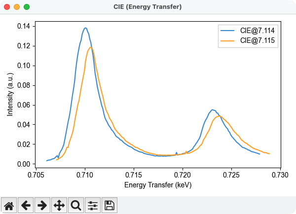
# Extract constant incident energy (CIE) cuts at 7.114 keV and 7.115 keV.
measurement.cut(mode="CIE", energies=[7.114, 7.115], widths=0.0005)
# Plot the map.
axes = measurement.plot()
ax1, ax2, *_ = axes.flatten()
ax1.set_title(r"Fe2O3 K$\alpha_1$K$\alpha_2$ RIXS")
ax1.figure.tight_layout()
plt.show()
Detailed Explanations#
Following the import statements, we create a logger to track the processing steps. By default, it is set to the INFO level, but you can change it to DEBUG for more detailed output.
logging.getLogger("daxs").setLevel(logging.INFO)
Next, we define the data mappings, which specify which datasets in the HDF5 file correspond to the different axes. We also specify the HDF5 filename and a selection of scan indices to be used for constructing the RIXS plane. Here 201 scans (4 to 224) are used.
data_mappings = {
    "x": ".1/measurement/hdh_energy",
    "y": ".1/instrument/positioners/xes_en",
    "signal": ".1/measurement/det_dtc_apd",
    "monitor": ".1/measurement/I02",
}
hdf5_filename = resources.getfile("Fe2O3_Ka1Ka2_RIXS.h5")
selection = "4-224"
With this information, we create an Hdf5Source object to read the specified scans from the HDF5 file. The source is then used to create a Rixs measurement object. Note that the scans will be used to construct a single plane.
source = Hdf5Source(hdf5_filename, selection, data_mappings=data_mappings)
measurement = Rixs(source)
As each scan is acquired at different sample positions, we correct for the inhomogeneous sample by applying concentration correction. Here, we use scan 225 as the reference scan. Since the number of points in the concentration correction scan is the same as the number of scans used to build the RIXS plane, the process is straightforward. The daxs library also includes a more advanced concentration correction method for cases when the number of points differ.
conc_corr_scan = 225
measurement.concentration_correction(conc_corr_scan)
Next, we plot the RIXS data, and get the axes for further customization.
axes = measurement.plot()
ax1, ax2 = axes.flatten()
ax1.set_title(r"Fe2O3 K$\alpha_1$K$\alpha_2$ RIXS")
ax1.figure.tight_layout()
plt.show()
Once the data is plotted it is easy to determine the position of relevant constant energy cuts. In this case we extract two cuts at incident energies of 7.114 keV and 7.115 keV, with a width of 0.5 eV. If we do the cuts before plotting, the points included in each of them will be automatically plotted on top of the map. The binned data for each cut is displayed in the second plot.
measurement.cut(mode="CIE", energies=[7.114, 7.115], widths=0.0005)
Below are the resulting plots.
A final note on the plot of the RIXS data: the map is replotted every time the view limits are changed, and the color scale is automatically adjusted based on the data range. Therefore, you can pan/zoom to specific regions of the plane, and the color scale will update accordingly, as shown in the animated plot above. This allows to explore low-intensity features that may be otherwise difficult to see.