X-ray Emission Spectroscopy Concentration Correction and Plotting#
This example demonstrates processing X-ray emission spectroscopy (XES) data, including concentration correction, outlier removal, normalization, and visualization.
import logging
import sys

import matplotlib.pyplot as plt

from daxs.measurements import Xes
from daxs.sources import Hdf5Source
from daxs.utils import resources

# Create a logger to track the processing steps.
logging.basicConfig(level=logging.INFO, stream=sys.stdout)
# The default level for the *daxs* logger is set to INFO.
# Increase to DEBUG to get more detailed output.
logging.getLogger("daxs").setLevel(logging.INFO)

# Define data mappings for XES data.
hdf5_filename = resources.getfile("A1_Kb_XES.h5")
data_mappings = {
    "x": ".1/measurement/xes_en",
    "signal": ".1/measurement/det_dtc_apd",
    "monitor": ".1/measurement/I02",
}

# Load data from scan 8.
source = Hdf5Source(hdf5_filename, 8, data_mappings=data_mappings)
measurement = Xes(source)

# Apply concentration correction using scan 9.
conc_corr_scan = 9
measurement.concentration_correction(conc_corr_scan)

# Detect and remove outliers.
measurement.find_outliers(threshold=9)
measurement.remove_outliers()

# Normalize by area.
measurement.normalize(mode="area")

# Plot the processed data.
ax = measurement.plot()

ax.set_xlabel("Energy (keV)")
ax.set_ylabel("Intensity (a.u.)")
ax.set_title("X-ray Emission Spectroscopy")

plt.tight_layout()
plt.show()
Detailed Explanations#
After the import statements and logging setup, we proceed to define the data mappings and load scan 8 from the HDF5 file and create an measurement from it.
hdf5_filename = resources.getfile("A1_Kb_XES.h5")
data_mappings = {
    "x": ".1/measurement/xes_en",
    "signal": ".1/measurement/det_dtc_apd",
    "monitor": ".1/measurement/I02",
}
source = Hdf5Source(hdf5_filename, 8, data_mappings=data_mappings)
measurement = Xes(source)
Next we apply concentration correction using the information from scan 9.
conc_corr_scan = 9
measurement.concentration_correction(conc_corr_scan)
The outliers are first detected using a modified threshold of 9 which will select only the most prominent outliers. After detection, the outliers are removed by calling the remove_outliers method.
measurement.find_outliers(threshold=9)
measurement.remove_outliers()
The data is then normalized by area to prepare it for visualization.
measurement.normalize(mode="area")
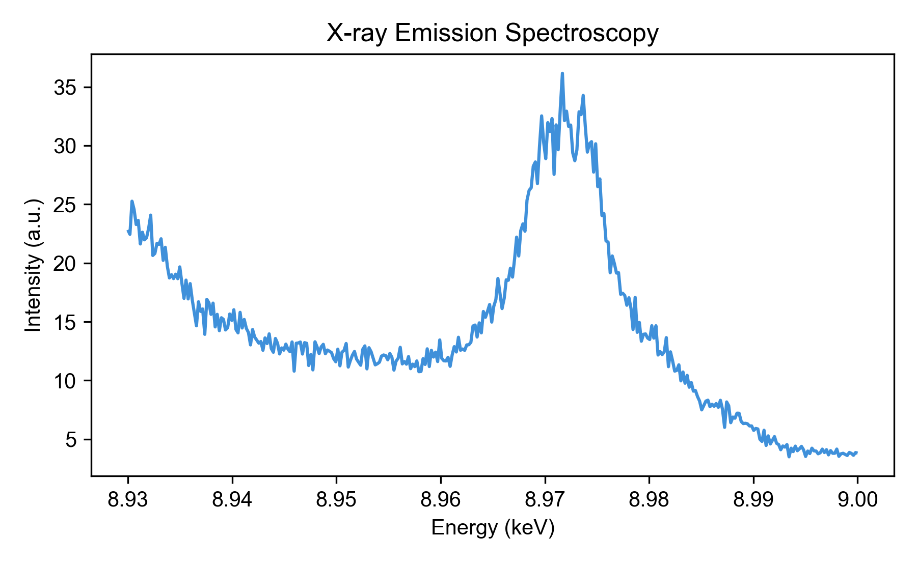
Finally, we plot the processed data using the built-in plot method. After recovering the axis, we set appropriate labels and title for clarity.
ax = measurement.plot()
ax.set_xlabel("Energy (keV)")
ax.set_ylabel("Intensity (a.u.)")
ax.set_title("X-ray Emission Spectroscopy")
plt.tight_layout()
plt.show()
The plot shows the corrected and normalized XES spectrum.