Plotting Separate X-ray Absorption Spectroscopy Measurements

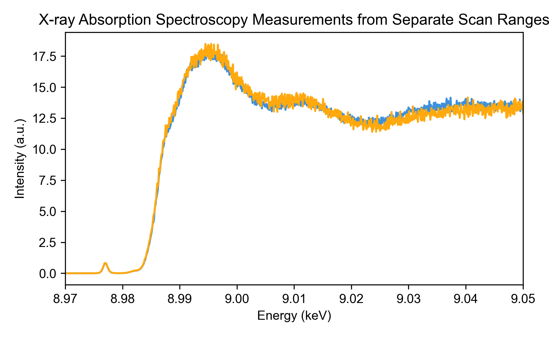
This example demonstrates how to process and visualize multiple X-ray absorption spectroscopy (XAS) scans from different ranges, including normalization and plotting for comparison.

import logging
import sys

import matplotlib.pyplot as plt

from daxs.measurements import Xas
from daxs.sources import Hdf5Source
from daxs.utils import resources

# Create a logger to track the processing steps.
logging.basicConfig(level=logging.INFO, stream=sys.stdout)
# The default level for the *daxs* logger is set to INFO.
# Increase to DEBUG to get more detailed output.
logging.getLogger("daxs").setLevel(logging.INFO)

# Define the data mappings used to process XAS data.
data_mappings = {
    "x": ".1/measurement/hdh_energy",
    "signal": [".1/measurement/det_dtc_apd"],
    "monitor": ".1/measurement/I02",
}

# Process and normalize measurements from separate scan ranges.
hdf5_filename = resources.getfile("CuCO3_Ka_XANES.h5")
measurements = []
for selection in ("1-4", "5-6"):
    source = Hdf5Source(hdf5_filename, selection, data_mappings=data_mappings)
    measurement = Xas(source)
    measurement.x = measurement.scans.get_common_axis("x", "intersection")
    measurement.normalize(mode="area")
    measurements.append(measurement)

# Plot the processed XAS data.
fig, ax = plt.subplots(figsize=(6, 3.7))

for _, measurement in enumerate(measurements):
    ax.plot(measurement.x, measurement.signal)

ax.set_title("X-ray Absorption Spectroscopy Measurements from Separate Scan Ranges")
ax.set_xlabel("Energy (keV)")
ax.set_ylabel("Intensity (a.u.)")
ax.set_xlim(8.97, 9.05)

plt.tight_layout()
plt.show()

Detailed Explanations

First, we import the necessary modules and we set up logging.

import logging
import sys

import matplotlib.pyplot as plt

from daxs.measurements import Xas
from daxs.sources import Hdf5Source
from daxs.utils import resources

# Create a logger to track the processing steps.
logging.basicConfig(level=logging.INFO, stream=sys.stdout)
# The default level for the *daxs* logger is set to INFO.
# Increase to DEBUG to get more detailed output.
logging.getLogger("daxs").setLevel(logging.INFO)

Next, we define the data mappings that specify which datasets in the HDF5 file correspond to the x-axis (incident energy), signal, and monitor for normalization.

data_mappings = {
    "x": ".1/measurement/hdh_energy",
    "signal": [".1/measurement/det_dtc_apd"],
    "monitor": ".1/measurement/I02",
}

We then load the HDF5 file and process measurements for two scan ranges (“1-4” and “5-6”). For each range, we create a data source and a measurement object, set a common x-axis across scans, normalize by area, and collect the measurements.

hdf5_filename = resources.getfile("CuCO3_Ka_XANES.h5")
measurements = []
for selection in ("1-4", "5-6"):
    source = Hdf5Source(hdf5_filename, selection, data_mappings=data_mappings)
    measurement = Xas(source)
    measurement.x = measurement.scans.get_common_axis("x", "intersection")
    measurement.normalize(mode="area")
    measurements.append(measurement)

Finally, we create a plot to visualize the normalized spectra from both scan ranges on the same axis for comparison.

fig, ax = plt.subplots(figsize=(6, 3.7))
for i, measurement in enumerate(measurements):
    ax.plot(measurement.x, measurement.signal)
ax.set_title("X-ray Absorption Spectroscopy Measurements from Separate Scan Ranges")
ax.set_xlabel("Energy (keV)")
ax.set_ylabel("Intensity (a.u.)")
ax.set_xlim(8.97, 9.05)
plt.tight_layout()
plt.show()

The resulting plot shows the processed XAS data, allowing comparison between different measurement sets.